Branded Figures and Tables in R and Python with Quarto

Quarto Version

This post was written and tested with Quarto CLI 1.9.37. Some APIs or behaviours may differ in earlier stable releases.

Quarto’s brand feature is a convenient way to keep a document’s look consistent across formats: define your colours, fonts, and logos once in a _brand.yml file, and everything from the navbar to the code blocks picks them up automatically. Code-generated outputs, however, are a different story. A ggplot2 scatter plot or a gt summary table will cheerfully ignore your brand and render with their own defaults. This post walks through one approach to close that gap: reading the resolved brand configuration at render time and applying it to every figure and table your code produces.

Key Principles

Quarto sets QUARTO_EXECUTE_INFO for every code cell; parse it for brand colours, fonts, and palettes.
Register web fonts before any plotting; graphics devices do not see brand-defined fonts by default.
Wrap the styling logic in theme_brand() (figures) and gt_brand() (tables) so every output inherits brand values.
Use renderings: [light, dark] and .light-content/.dark-content to match the reader’s selected theme automatically.
The companion repository mcanouil/quarto-brand-renderings has production-ready implementations with full error handling.

1 The Problem

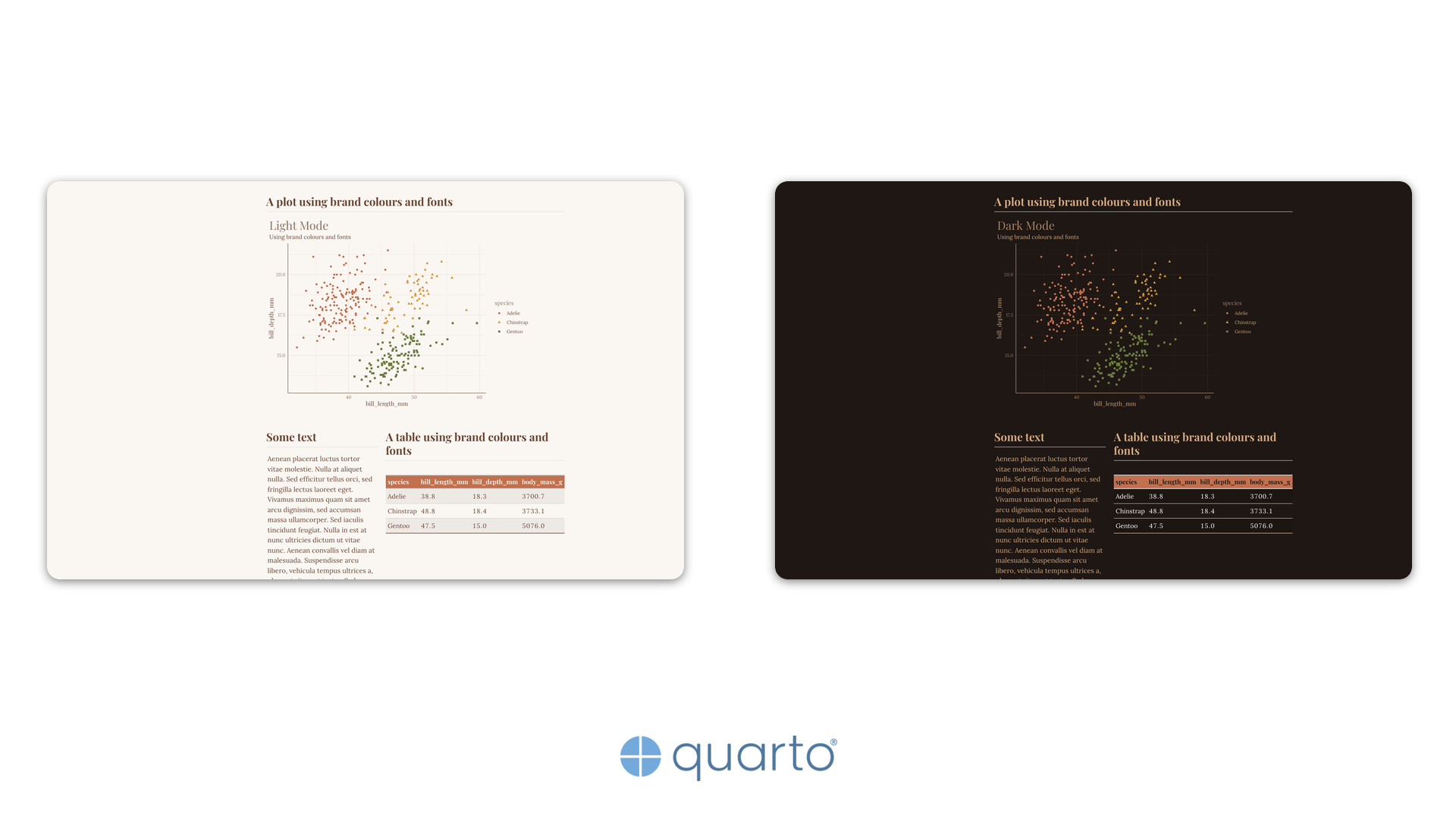
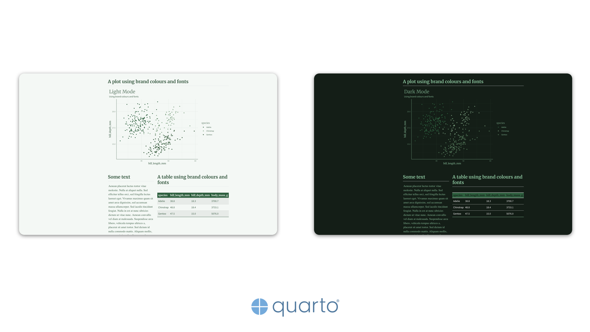
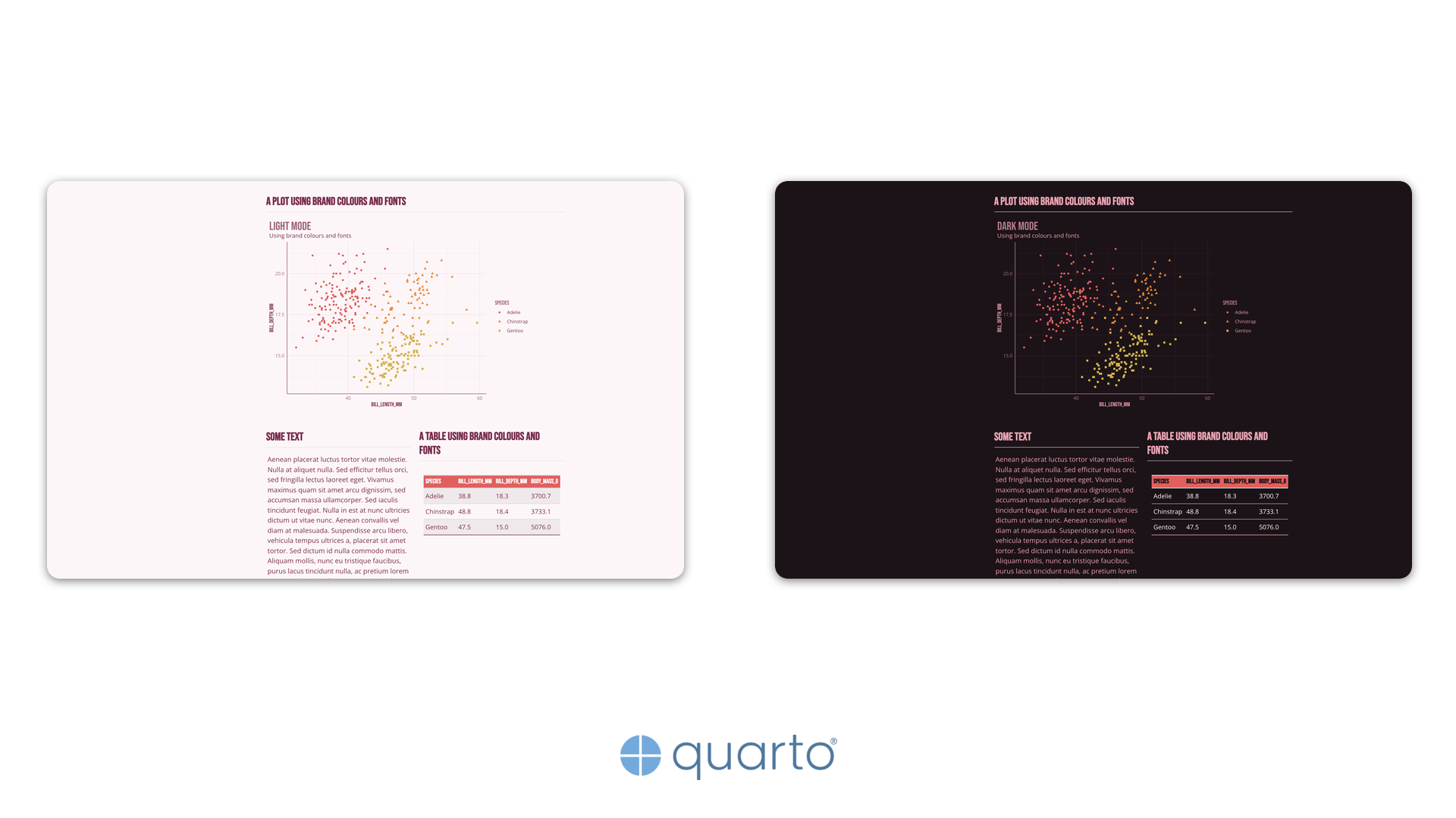
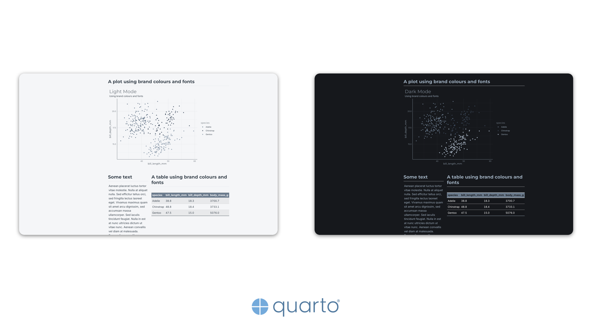
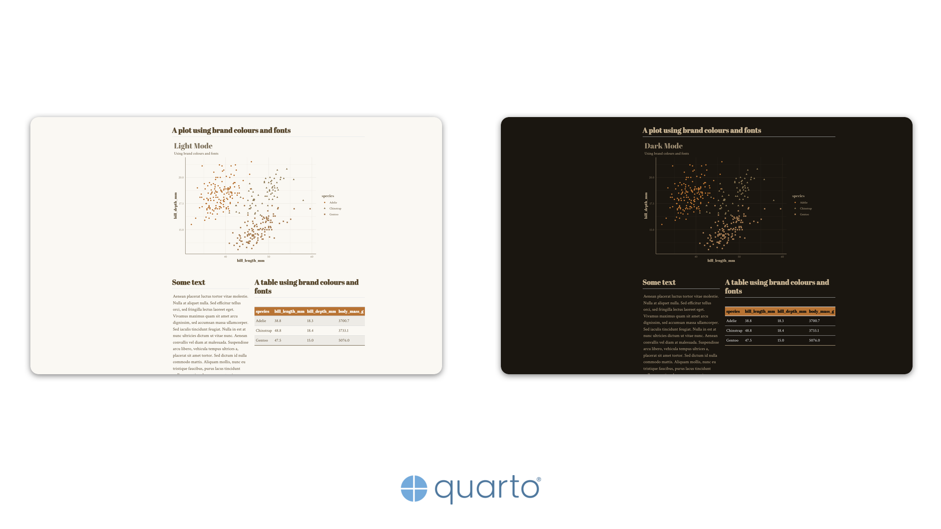
The goal is to make every visual output match the document’s brand without hardcoding hex values or font names. Here is what branded outputs look like across six different brand configurations, each with light and dark variants:

Alternative Approaches

There is no single right way to achieve branded outputs in R and Python. The brand.yml project provides dedicated R and Python packages that read a _brand.yml file directly and are the recommended starting point for most projects. At the time of writing, however, the brand.yml packages do not support font registration for graphics devices. You could also write your own wrappers, hard-code a shared palette, or use any other strategy that suits your workflow. This post demonstrates one particular approach: reading the resolved brand data from QUARTO_EXECUTE_INFO at render time, making it independent of external packages and portable across languages, with full font registration support.

2 The `QUARTO_EXECUTE_INFO` Approach

When Quarto renders a document, it sets the QUARTO_EXECUTE_INFO environment variable for every code cell. This variable points to a JSON file containing document metadata, format settings, and, crucially, the resolved brand configuration.

The brand data lives at format.render.brand in the JSON, with separate entries for each colour mode (light, dark). Reading it requires only a JSON parser.

get_brand_info <- function() {
2  jsonlite::fromJSON(
1    Sys.getenv("QUARTO_EXECUTE_INFO", unset = "")
  )
}

1: Read the environment variable set by Quarto.
2: Parse the JSON string into an R list.

import json
import os
import pathlib

def get_brand_info() -> dict:
1    raw = os.environ.get("QUARTO_EXECUTE_INFO", "")
    if not raw:
        return {}
    path = pathlib.Path(raw)
2    if path.is_file():
        return json.loads(path.read_text())
    return json.loads(raw)

1: Read the environment variable set by Quarto.
2: The value may be a file path or a raw JSON string; check which.

Exploring the Structure

During development, print the full JSON to see what is available:

info <- get_brand_info()
cat(jsonlite::toJSON(info[["format"]][["render"]][["brand"]], pretty = TRUE))

info = get_brand_info()
print(json.dumps(info["format"]["render"]["brand"], indent=2))

3 Brand Data Structure

The brand object under format.render.brand contains one entry per colour mode. Each mode holds a data object with colour and typography definitions.

{
  "light": {
    "data": {
      "color": {
        "palette": {
          "anchor-blue": "#2f5d8a",
          "harbour-teal": "#2d8c8f",
          "strait-violet": "#5f6fb3"
        },
        "foreground": "#4f789e",
        "background": "#f8fafc"
      },
      "typography": {
        "base": "Chakra Petch",
        "headings": "Great Vibes",
        "monospace": "JetBrains Mono",
        "fonts": [
          { "family": "Chakra Petch", "source": "bunny" }
        ]
      }
    }
  },
  "dark": {
    "data": { "..." }
  }
}

The key fields are:

color.palette: named colour values used for data series and accents.
color.foreground / color.background: ink and paper colours for the given mode.
typography.base / typography.headings: font family names.
typography.fonts: font specifications including source (bunny, google, file, or system).

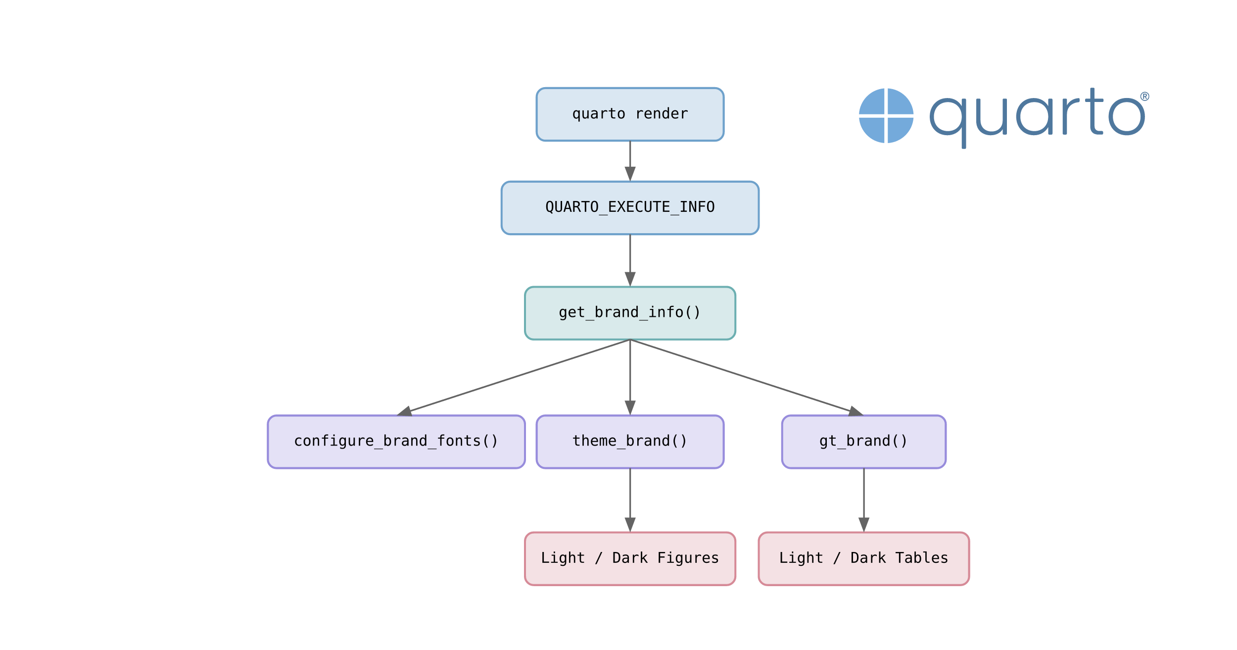
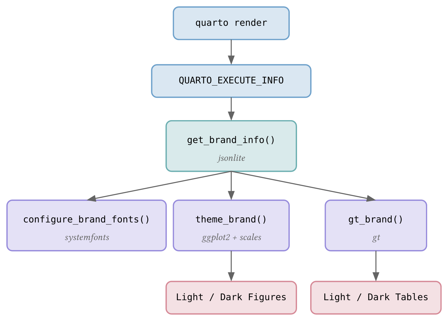
The diagrams below summarise how each helper function fits into the rendering pipeline.

Figure 1: R workflow for branded figures and tables.

Figure 2: Python workflow for branded figures and tables.

4 Dependencies

This approach relies on a handful of packages for each language.

jsonlite: parse the QUARTO_EXECUTE_INFO JSON.
ggplot2: the ink, paper, accent, and palette.* theme elements used by theme_brand() are not yet on CRAN.
gt: table styling.
scales: colour blending via col_mix().
systemfonts: font discovery, registration, and web font embedding for SVG output.

plotnine: ggplot2-style plotting.
great_tables: table styling.
polars: data manipulation.
pyfonts: font loading from Bunny Fonts and Google Fonts, created by Joseph Barbier. The companion repository uses a development version of pyfonts for improved font subset selection.

5 Font Registration

Web fonts defined in a brand configuration are not available to R or Python graphics devices by default. Before creating any plots or tables, a configure_brand_fonts() function registers each font so that graphics devices can find them. Call it once in a setup chunk at the top of your document.

The systemfonts package handles font discovery and registration.

configure_brand_fonts <- function(brand_mode = "light") {
  info <- get_brand_info()
  brand <- info[["format"]][["render"]][["brand"]]
1  doc_dir <- dirname(info[["document-path"]])

  for (mode in intersect(c("light", "dark"), names(brand))) {
    fonts <- brand[[mode]][["data"]][["typography"]][["fonts"]]
    for (ifont in seq_len(nrow(fonts))) {
      family <- fonts[["family"]][[ifont]]
      source <- fonts[["source"]][[ifont]]

      if (identical(source, "file")) {
        files <- fonts[["files"]][[ifont]]
        for (fp in as.character(files[["path"]])) {
2          resolved <- file.path(doc_dir, fp)
3          systemfonts::register_font(family, plain = resolved)
        }
      } else {
4        systemfonts::require_font(family, repositories = "Bunny Fonts")
      }
    }
  }
5  systemfonts::reset_font_cache()
}

1: Resolve the document directory from QUARTO_EXECUTE_INFO for relative font paths.
2: Build the full path to each local font file.
3: Register local font files with systemfonts::register_font().
4: Download web fonts from Bunny Fonts (or Google Fonts) with systemfonts::require_font().
5: Reset the font cache so newly registered fonts become available.

The matplotlib.font_manager module handles font registration, with pyfonts for downloading web fonts.

import matplotlib.font_manager as fm
import pyfonts

def configure_brand_fonts() -> None:
    info = get_brand_info()
    brand = info["format"]["render"]["brand"]
1    doc_dir = pathlib.Path(info["document-path"]).parent

    for mode in ["light", "dark"]:
        if mode not in brand:
            continue
        fonts = brand[mode]["data"]["typography"]["fonts"]
        for font_spec in fonts:
            family = font_spec["family"]
            source = font_spec["source"]

            if source == "file":
                for f in font_spec.get("files", []):
2                    resolved = doc_dir / f["path"]
3                    fm.fontManager.addfont(str(resolved))
            elif source in ("bunny", "google"):
                if source == "bunny":
                    props = pyfonts.load_bunny_font(family)
                else:
                    props = pyfonts.load_google_font(family)
4                fm.fontManager.addfont(props.get_file())

1: Resolve the document directory for relative font paths.
2: Build the full path to each local font file.
3: Register local font files with matplotlib.font_manager.
4: Download web fonts using pyfonts and register them.

SVG Font Rendering

When generating figures as SVG, the SVG files must be inlined directly into the HTML page for fonts to render correctly. An SVG file referenced via an <img> tag is treated as an isolated document by the browser: it cannot access the page’s stylesheets or @import rules, so any @font-face declarations inside the SVG that reference external URLs are silently ignored. Inlining the SVG into the page DOM removes this boundary, allowing the browser to resolve font imports just like any other CSS resource.

The companion repository includes an inline-svglite.lua Lua filter that replaces <img> references with raw SVG content automatically. See the companion repository for the full implementation.

6 Branded Figures

The theme_brand() function extracts colours and fonts from the brand data and builds a complete ggplot2 or plotnine theme. The idea is straightforward: pull out the ink (foreground), paper (background), and palette colours, then pass them to the theme constructor. In R, the latest ggplot2 supports ink, paper, and accent parameters directly in theme_minimal(); in Python, each theme element is styled individually.

theme_brand <- function(base_size = 11, brand_mode = "light") {
  info <- get_brand_info()
  brand <- info[["format"]][["render"]][["brand"]]
  brand_data <- brand[[brand_mode]][["data"]]
  colors <- brand_data[["color"]]
  typography <- brand_data[["typography"]]
1  palette_values <- unname(unlist(colors[["palette"]]))

2  ink <- colors[["foreground"]]
  paper <- colors[["background"]]
3  accent <- scales::col_mix(ink, paper, amount = 0.25)

  ggplot2::theme_minimal(
    base_size = base_size,
4    base_family = typography[["base"]],
    header_family = typography[["headings"]],
5    ink = ink,
    paper = paper,
    accent = accent
  ) +
    ggplot2::theme(
      plot.title = ggplot2::element_text(
        colour = accent,
        size = ggplot2::rel(2)
      ),
6      palette.colour.discrete = palette_values,
      palette.fill.discrete = palette_values
    )
}

1: Flatten the named palette into a character vector.
2: Extract foreground (ink) and background (paper) from the brand colours.
3: Blend ink and paper to create an accent colour for titles and axes.
4: Apply brand fonts to body text and headings.
5: Pass ink, paper, and accent to theme_minimal().
6: Set the discrete colour palette for geoms.

R uses scales::col_mix() to blend colours. Python needs a small helper since there is no equivalent in plotnine:

def _col_mix(a: str, b: str, amount: float = 0.25) -> str:
    ra, ga, ba = int(a[1:3], 16), int(a[3:5], 16), int(a[5:7], 16)
    rb, gb, bb = int(b[1:3], 16), int(b[3:5], 16), int(b[5:7], 16)
    r = int(ra + (rb - ra) * amount)
    g = int(ga + (gb - ga) * amount)
    b_val = int(ba + (bb - ba) * amount)
    return f"#{r:02x}{g:02x}{b_val:02x}"

Because plotnine does not support palette.* theme elements, a separate helper extracts the colour palette for use with scale_color_manual():

def get_brand_palette(brand_mode: str = "light") -> list[str]:
    info = get_brand_info()
    brand = info["format"]["render"]["brand"]
    palette = brand[brand_mode]["data"]["color"]["palette"]
    return list(palette.values())

from plotnine import (
    element_line, element_rect, element_text, theme, theme_minimal
)

def theme_brand(base_size: int = 11, brand_mode: str = "light") -> theme:
    info = get_brand_info()
    brand = info["format"]["render"]["brand"]
    brand_data = brand[brand_mode]["data"]
    colors = brand_data["color"]
    typography = brand_data["typography"]

1    ink = colors["foreground"]
    paper = colors["background"]
2    accent = _col_mix(ink, paper, 0.25)
    base_family = typography["base"]
    heading_family = typography["headings"]

    base_line_size = base_size / 22
    grid_major_colour = _col_mix(ink, paper, 0.8)
    grid_minor_colour = _col_mix(ink, paper, 0.9)

    return theme_minimal(
        base_size=base_size,
3        base_family=base_family
    ) + theme(
        plot_background=element_rect(fill=paper, colour="none"),
        panel_background=element_rect(fill=paper, colour="none"),
        panel_grid_major=element_line(colour=grid_major_colour, size=base_line_size),
        panel_grid_minor=element_line(colour=grid_minor_colour, size=base_line_size * 0.5),
        text=element_text(colour=ink),
        axis_title=element_text(family=heading_family),
        axis_line_x=element_line(colour=accent),
        axis_line_y=element_line(colour=accent),
        plot_title=element_text(
            family=heading_family,
            colour=accent,
            size=base_size * 2,
        ),
        plot_subtitle=element_text(colour=ink),
        legend_title=element_text(family=heading_family, colour=accent),
        legend_background=element_rect(fill=paper, colour="none"),
    )

1: Extract foreground (ink) and background (paper) from the brand colours.
2: Blend ink and paper to create an accent colour (custom _col_mix() helper).
3: Apply brand fonts to body text and headings.

Note

The latest version of ggplot2 supports ink, paper, accent, and palette.* theme elements natively. plotnine does not have these parameters, so each element must be styled individually.

Companion Repository

The code samples in this post are intentionally simplified. The companion repository contains production-ready versions with full error handling, defensive .get() fallbacks, and additional styling such as continuous palette support in R.

6.1 Usage

With theme_brand() defined, applying it to a plot is straightforward.

library(ggplot2)
penguins <- read.csv("penguins.csv")

ggplot(penguins) +
  aes(x = bill_length_mm, y = bill_depth_mm, colour = species) +
  geom_point(na.rm = TRUE) +
  theme_brand(brand_mode = "light") +
  labs(title = "Light Mode", subtitle = "Using brand colours and fonts")

import polars as pl
from plotnine import aes, geom_point, ggplot, labs, scale_color_manual

penguins = pl.read_csv("penguins.csv", null_values="NA").drop_nulls(
    ["bill_length_mm", "bill_depth_mm"]
)

palette = get_brand_palette("light")

(
    ggplot(penguins.to_pandas())
    + aes(x="bill_length_mm", y="bill_depth_mm", color="species")
    + geom_point()
    + theme_brand(brand_mode="light")
    + scale_color_manual(values=palette)
    + labs(title="Light Mode", subtitle="Using brand colours and fonts")
)

7 Branded Tables

The gt_brand() function follows the same pattern: extract brand colours and fonts, then apply them to the table. Column headers get the first palette colour as a background, body borders use an accent derived from blending ink and paper, and the base and heading fonts are applied throughout.

gt_brand <- function(data, brand_mode = "light") {
  info <- get_brand_info()
  brand <- info[["format"]][["render"]][["brand"]]
  brand_data <- brand[[brand_mode]][["data"]]
  colors <- brand_data[["color"]]
  typography <- brand_data[["typography"]]
  palette <- unname(unlist(colors[["palette"]]))

  ink <- colors[["foreground"]]
  paper <- colors[["background"]]
  accent <- scales::col_mix(ink, paper, amount = 0.25)

  gt::gt(data) |>
1    gt::opt_table_font(font = typography[["base"]]) |>
    gt::tab_options(
2      table.background.color = paper,
      table.font.color = ink,
3      column_labels.background.color = palette[[1L]],
      column_labels.font.weight = "bold",
4      table_body.border.top.color = accent,
      table_body.border.bottom.color = accent
    ) |>
    gt::tab_style(
5      style = gt::cell_text(font = typography[["headings"]], color = paper),
      locations = gt::cells_column_labels()
    )
}

1: Set the base font for the entire table.
2: Apply brand background and text colours.
3: Use the first palette colour for column header background.
4: Use the accent colour for table body borders.
5: Style column labels with the heading font and contrasting colour.

from great_tables import GT, loc, style

def gt_brand(data, brand_mode: str = "light") -> GT:
    info = get_brand_info()
    brand = info["format"]["render"]["brand"]
    brand_data = brand[brand_mode]["data"]
    colors = brand_data["color"]
    typography = brand_data["typography"]
    palette = list(colors["palette"].values())

    ink = colors["foreground"]
    paper = colors["background"]
    accent = _col_mix(ink, paper, 0.25)

    return (
        GT(data)
        .tab_options(
1            table_font_names=typography["base"],
2            table_font_color=ink,
            table_background_color=paper,
3            column_labels_background_color=palette[0] if palette else accent,
            column_labels_font_weight="bold",
4            table_body_border_top_color=accent,
            table_body_border_bottom_color=accent,
        )
        .tab_style(
            style=style.text(
                font=typography["headings"],
                color=paper,
5                weight="bold",
            ),
            locations=loc.column_labels(),
        )
    )

1: Set the base font for the entire table.
2: Apply brand background and text colours.
3: Use the first palette colour for column header background.
4: Use the accent colour for table body borders.
5: Style column labels with the heading font and contrasting colour.

8 Light and Dark Mode

Quarto supports light and dark colour modes, and the brand data includes separate colour definitions for each. The helper functions accept a brand_mode parameter to select which variant to use.

For figures, Quarto’s renderings cell option generates both variants from a single code cell.

#| renderings: [light, dark]

The code loops over both modes and prints each plot. Quarto then displays the correct one based on the reader’s selected theme.

For tables, use Quarto’s .light-content and .dark-content CSS classes to conditionally display the appropriate version.

::: {.light-content}
Table rendered with `brand_mode = "light"`.
:::

::: {.dark-content}
Table rendered with `brand_mode = "dark"`.
:::

Automatic Theme Matching

Combining renderings: [light, dark] with branded themes means figures and tables automatically match the reader’s selected theme without any JavaScript.

9 Putting It All Together

The full workflow boils down to four steps:

Call configure_brand_fonts() once in a hidden setup chunk (#| include: false) to register brand fonts before any plotting.
Apply theme_brand(brand_mode = ...) to every ggplot2 or plotnine figure.
Pass your data through gt_brand(data, brand_mode = ...) for every gt or great_tables table.
Use renderings: [light, dark] on figure cells and .light-content/.dark-content divs on tables so the reader’s theme preference is respected automatically.

That is the entire pattern. Every helper reads from the same QUARTO_EXECUTE_INFO source, so switching to a different brand configuration is just a matter of changing your _brand.yml file; no code changes are needed.

10 Conclusion

The QUARTO_EXECUTE_INFO environment variable provides language-agnostic access to Quarto’s resolved brand configuration at render time. With a small set of helper functions, you can apply consistent brand colours, fonts, and palettes to every figure and table your code produces.

This is one approach among several (see the note on brand.yml packages above), but it has the advantage of working identically in R and Python, supporting full font registration, and requiring no dependencies beyond a JSON parser and the plotting libraries you are already using. Browse the companion repository for six complete brand configurations with production-ready implementations, and feel free to adapt the helpers to your own projects.

11 Further Resources

Multiformat Branding with _brand.yml: the official Quarto documentation on the brand feature.
Execution Context Information: how QUARTO_EXECUTE_INFO works and what data it exposes.
Execution Options: code cell options including renderings for light/dark mode.
HTML Theming: customising HTML themes, Sass variables, and dark mode support.
brand.yml Specification: the full specification and documentation for _brand.yml files.

Reuse

CC BY-NC-SA 4.0

Citation

BibTeX citation:

@misc{canouil2026,
  author = {CANOUIL, Mickaël},
  title = {Branded {Figures} and {Tables} in {R} and {Python} with
    {Quarto}},
  date = {2026-04-15},
  url = {https://mickael.canouil.fr/posts/2026-04-15-quarto-brand-figures-tables/},
  langid = {en-GB}
}

For attribution, please cite this work as:

CANOUIL, M. (2026, April 15). Branded Figures and Tables in R and Python with Quarto. Mickael.canouil.fr. https://mickael.canouil.fr/posts/2026-04-15-quarto-brand-figures-tables/

1 The Problem

2 The QUARTO_EXECUTE_INFO Approach

3 Brand Data Structure

4 Dependencies

5 Font Registration

6 Branded Figures

6.1 Usage

7 Branded Tables

8 Light and Dark Mode

9 Putting It All Together

10 Conclusion

11 Further Resources

Reuse

Citation

2 The `QUARTO_EXECUTE_INFO` Approach