Gribouille: a Grammar of Graphics for Typst

Skip to main content

1 Introduction

Typst has grown from a curious newcomer to a credible alternative for scientific writing, reports, and slide decks. What it still lacked, until today, was a real grammar of graphics: a way to declare a figure with the same vocabulary you would reach for in ggplot2, then have it draw, lay out, and align with the rest of the document.

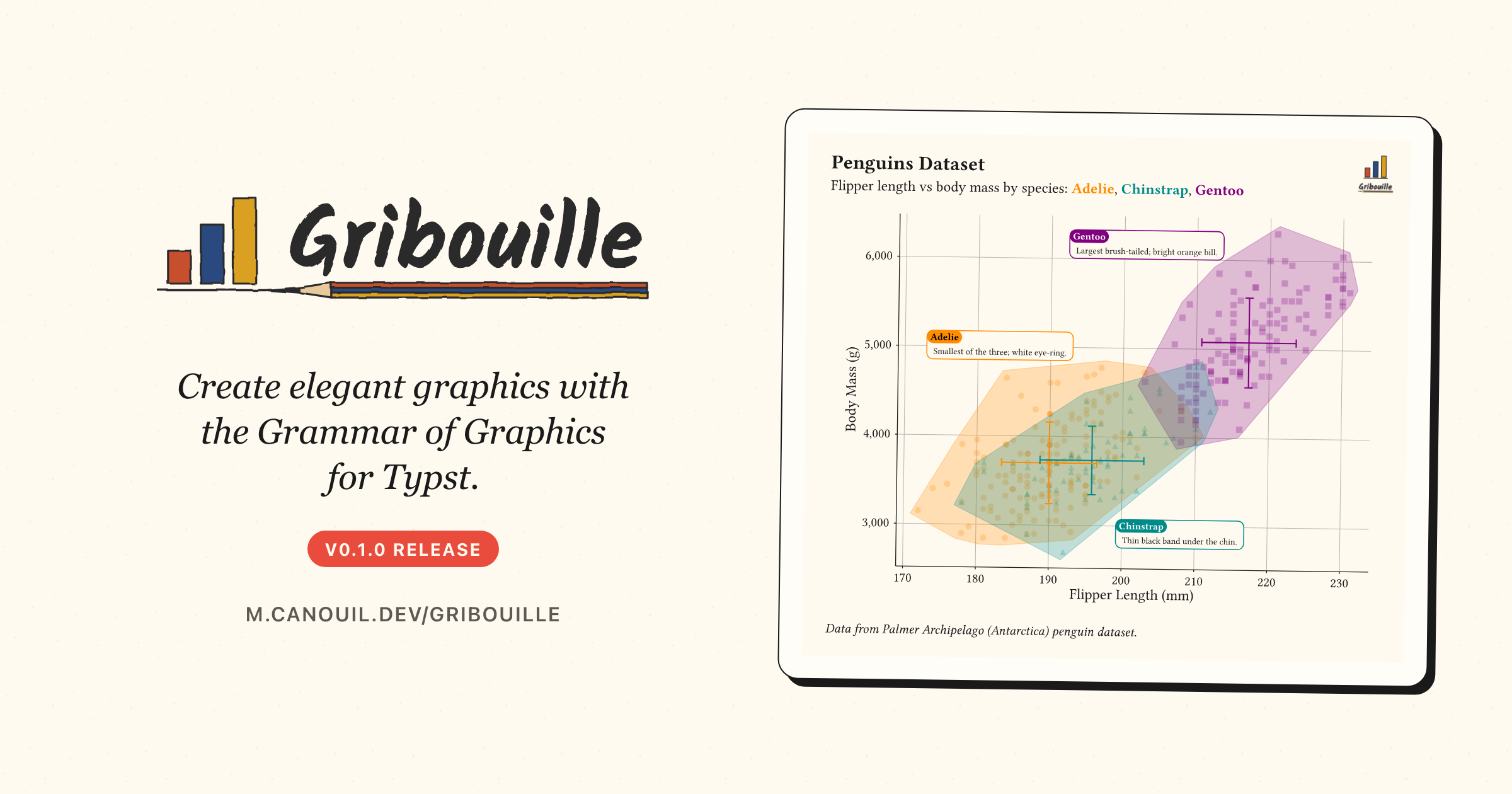
Gribouille (French for scribble) is the first cut of that library. Version 0.1.0 lands on Typst Universe with this announcement, modelled closely on ggplot2, drawing on top of cetz, and shipped with a documentation site that is itself a Quarto project rendered by the quarto-typst-render extension. Every figure in this post is a real, freshly compiled plot.

NoteAt a glance

• Gribouille v0.1.0 on Typst Universe: #import "@preview/gribouille:0.1.0": *.
• A broad library of geoms and stats, scales spanning every aesthetic, a range of built-in themes, and full facet support.
• compose() orchestrates several plots into a single figure with a shared, hoisted legend, fed by a new defer: true flag on plot().
• quarto-typst-render v0.13.1 ships typst_define(), the Python and R helper that streams arbitrary values, scalars, lists, dictionaries, and full data frames alike, straight into Typst code blocks.

2 Why a grammar of graphics for Typst

Until now, producing a figure inside a Typst document meant taking a detour through another language. You would leave Typst to call out to ggplot2, matplotlib, or plotnine, save a PNG or SVG, and import it back. That works, but it splits the toolchain in two: one font system on the page, another inside the figure; one colour palette in the report, another in the chart; one render pass that knows about the layout, another that does not.

cetz already gives Typst a robust low-level drawing API, but the declarative layer that turns a dataset, a mapping, and a few layers into a publication-quality figure was missing. That is exactly the gap Gribouille fills.

One toolchain. Same fonts, same palette, same render pass, from data to PDF.

The pay-off is a single toolchain. Give a plot an alt: description and Gribouille wraps the result in a Typst figure element with kind: "gribouille-plot", so you can attach show rules, captions, or cross-references in one place; with or without it, every plot shares the document’s fonts, palette, and geometry. The YAML front-matter of this very post wires its background: and foreground: to the site’s light and dark colours, and every figure below reacts automatically when you toggle the theme. Compilation is deterministic, offline-friendly, and produces a PDF straight out of Typst with no Python or R runtime required.

3 A respectful nod to ggplot2

A short personal aside. I have been using ggplot2 since almost its first release, and a large part of how I think about data visualisation comes from that work. This release would not exist without Hadley Wickham’s original vision, nor without the people carrying it forward today, in particular Thomas Lin Pedersen and Teun van den Brand, and the wider community of contributors who keep shaping the package through to the recent v4 release.

Gribouille is, in many ways, a port of ggplot2’s vocabulary into Typst. The names line up: plot() instead of ggplot(), geom-point() for geom_point(), facet-wrap(), scale-colour-*(), theme-minimal(), and so on. Where the two part ways, it is because Typst is a different language, with no lazy evaluation, no plot object you can mutate after the fact, and no ggsave() output pipeline. Column names are plain strings. Per-aesthetic type coercion is done inline with as-factor() and as-numeric(). These are opinionated departures, but the mental model is the same one you already have.

4 Build a penguins plot, one layer at a time

The library ships the Palmer Penguins dataset under the penguins symbol. The walk-through below builds a single figure end to end, one grammar concept at a time, with brief notes on alternatives at each step. It is a tighter version of the Get Started page on the documentation site.

Every plot you build composes the same pieces. plot() wraps a stack of layers, each sheet sitting on the one below, from data and mapping at the foundation up through theme and labels.

The post’s YAML points the typst-render extension at a one-line preamble file so every {typst} block has the library in scope:

extensions:
  typst-render:
    preamble: _preamble.typ

And _preamble.typ contains:

#import "@preview/gribouille:0.1.0": *

You would write the same #import once at the top of your own Typst document.

4.1 Data and aesthetics

Every plot starts with a dataset and an aes() mapping that binds column names to visual channels. At a minimum, geom-point() needs x and y.

#plot(
  data: penguins,
  mapping: aes(x: "flipper-len", y: "body-mass"),
  layers: (geom-point(size: 2pt),),
  width: 12cm,
  height: 9cm,
)

The plot-level mapping is inherited by every layer. If only one layer needs a given mapping, you can also pass it inside that layer’s mapping: argument and keep the plot-level mapping minimal.

4.2 Encode a third variable with colour

Add colour: "species" and the points split visually by group.

#plot(
  data: penguins,
  mapping: aes(
    x: "flipper-len",
    y: "body-mass",
    colour: "species",
  ),
  layers: (geom-point(size: 2pt, alpha: 0.85),),
  width: 12cm,
  height: 9cm,
)

If your figure must remain legible in greyscale, swap colour: "species" for shape: "species" and the same grouping rides the point shape instead. Both aesthetics can be combined when accessibility matters.

#plot(
  data: penguins,
  mapping: aes(
    x: "flipper-len",
    y: "body-mass",
    shape: "species",
  ),
  layers: (geom-point(size: 2pt, alpha: 0.85),),
  width: 12cm,
  height: 9cm,
)

4.3 Stack a second layer

Layers stack in the order you list them. Adding geom-smooth() draws one fitted line per colour group, because the colour aesthetic is inherited from the plot-level mapping.

Note

Only method: "lm" is supported in this release; LOESS is deferred for the reason listed in the limitations section.

#plot(
  data: penguins,
  mapping: aes(
    x: "flipper-len",
    y: "body-mass",
    colour: "species",
    fill: "species",
  ),
  layers: (
    geom-point(size: 2pt, alpha: 0.6),
    geom-smooth(method: "lm", alpha: 0.2),
  ),
  width: 12cm,
  height: 9cm,
)

4.4 Pick a palette

scale-colour-discrete() replaces the default palette. A matching scale-fill-discrete() keeps the confidence ribbons in step with the points.

#let cb = (
  rgb("#0072B2"),
  rgb("#D55E00"),
  rgb("#009E73"),
)

#plot(
  data: penguins,
  mapping: aes(
    x: "flipper-len",
    y: "body-mass",
    colour: "species",
    fill: "species",
  ),
  layers: (
    geom-point(size: 2pt, alpha: 0.6),
    geom-smooth(method: "lm", alpha: 0.2),
  ),
  scales: (
    scale-colour-discrete(palette: cb),
    scale-fill-discrete(palette: cb),
  ),
  width: 12cm,
  height: 9cm,
)

Tip

scale-colour-okabe-ito() exposes the same Okabe-Ito palette used in the example but as a one-liner if you do not want to spell out the colour codes.

4.5 Split into small multiples

facet-wrap() lays out one panel per level of a discrete column, sharing scales across panels.

#let cb = (
  rgb("#0072B2"),
  rgb("#D55E00"),
  rgb("#009E73"),
)

#plot(
  data: penguins,
  mapping: aes(
    x: "flipper-len",
    y: "body-mass",
    colour: "species",
    fill: "species",
  ),
  layers: (
    geom-point(size: 2pt, alpha: 0.6),
    geom-smooth(method: "lm", alpha: 0.2),
  ),
  scales: (
    scale-colour-discrete(palette: cb),
    scale-fill-discrete(palette: cb),
  ),
  facet: facet-wrap("island"),
  width: 12cm,
  height: 9cm,
)

Tip

For two crossed factors, facet-grid() produces a matrix of panels instead.

4.6 Polish

A theme, axis labels, and the figure is ready for the page.

format-comma(), passed to scale-y-continuous(labels: ...), turns 5000 into 5,000 on the y-axis. Sibling helpers cover number, percent, currency, scientific notation, and case or wrap formatting.

element-typst() wires the subtitle to render as Typst markup, so the linear-fit formula $hat(y) = beta_0 + beta_1 dot.c x$ and the per-species names appear with maths and inline colour without leaving the string.

A single species-colours dictionary feeds both scale-colour-discrete() (limits: plus palette:) and the second subtitle line. The entries are mapped to coloured #text(...) snippets, joined into one Typst-markup string.

Legend placement is controlled with guides() bound to guide-legend(position: ...). position: accepts the side strings "top", "right", "bottom", "left", a Typst alignment like bottom + right for an inside-panel corner, or a (dx:, dy:) offset for arbitrary placement.

The same constructor exposes direction, byrow, nrow, and ncolumn for swatch layout, and a "top" or "bottom" placement automatically lays a colourbar or size ladder out horizontally. The ncol argument was renamed to ncolumn in the run-up to this release, so older snippets need updating before they compile.

#let species-colours = (
  Adelie:    rgb("#0072B2"),
  Chinstrap: rgb("#D55E00"),
  Gentoo:    rgb("#009E73"),
)

#plot(
  data: penguins,
  mapping: aes(
    x: "flipper-len",
    y: "body-mass",
    colour: "species",
    fill: "species",
    shape: "species",
  ),
  layers: (
    geom-point(size: 2pt, alpha: 0.6),
    geom-smooth(method: "lm", alpha: 0.2),
  ),
  scales: (
    scale-colour-discrete(
      limits: species-colours.keys(),
      palette: species-colours.values(),
    ),
    scale-fill-discrete(
      limits: species-colours.keys(),
      palette: species-colours.values(),
    ),
    scale-y-continuous(labels: format-comma()),
  ),
  facet: facet-wrap("island"),
  guides: guides(
    colour: guide-legend(position: bottom + right),
    fill: guide-legend(position: bottom + right),
    shape: guide-legend(position: bottom + right),
  ),
  labs: labs(
    title: "Penguin Body Mass Scales with Flipper Length",
    subtitle: {
      [Linear fit $hat(y) = beta_0 + beta_1 dot.c x$ on every island for three species: ]
      species-colours.pairs()
        .map(p => text(fill: p.at(1), weight: "bold", p.at(0)))
        .join(", ")
    },
    x: "Flipper Length (mm)",
    y: "Body Mass (g)",
    colour: "Species",
    fill: "Species",
    shape: "Species",
  ),
  theme: theme-minimal(
    plot-title: element-text(size: 12pt, weight: "bold"),
    plot-subtitle: element-typst(size: 9pt),
  ),
  width: 12cm,
  height: 9cm,
)

5 Compose multiple plots

Sometimes a story needs more than one panel. compose() takes several deferred plots, lays them out on a grid or stack, and hoists their shared legend into a single guide block at the edge of the figure. The deferred plots are produced by passing defer: true to plot(), which returns a spec dictionary instead of rendering immediately.

Many plots, one legend. compose() hoists the shared aesthetics for you.

#let panel(mapping) = plot(
  data: penguins,
  mapping: mapping,
  layers: (geom-point(size: 2pt, alpha: 0.85),),
  width: 6cm,
  height: 4.5cm,
  defer: true,
)

#compose(
  panel(aes(x: "flipper-len", y: "body-mass", colour: "species")),
  panel(aes(x: "bill-len", y: "body-mass", colour: "species")),
  layout: "grid",
  columns: 1,
)

TipHoisting knobs

The hoisting is configurable. collect: controls which aesthetics are merged: auto hoists every legend identical across panels, none keeps each panel’s own legend in place, and an array such as ("colour",) whitelists specific aesthetics. guides-placement: sits the shared legend on "right", "left", "top", or "bottom". layout: switches between "grid" (with columns: and gutter:) and "stack" (with direction: such as ttb or ltr).

Note

You only need compose() when you want the shared legend hoisted. A rendered plot is ordinary Typst content, so the base grid and stack functions arrange several plots just as well when each keeps its own legend.

6 Drive Gribouille from any computation

Typst Render 0.13.1 adds a small but powerful helper called typst_define(), available from both R and Python. It lets a code cell hand any value to every {typst} block in the document under a single Typst dictionary named typst_define. A scalar, a list, a dictionary, a NumPy array, a Polars DataFrame, anything JSON-serialisable, lands in Typst as the corresponding native value.

Compute anywhere, render in Typst. typst_define() is the bridge.

The mechanism is deliberately plain. The helper serialises the values you give it to JSON, hex-encodes them, and emits a tiny Pandoc metadata block of the form ---\ntypst-define: <hex>\n---\n. The extension’s Lua filter, which runs at the pre-quarto stage, decodes that block and injects a #let typst_define = (...) preamble in front of every Typst compilation. You compute on one side, read typst_define.something on the other, and the two stay in step regardless of which language did the work.

That bridge is what makes the rest of this section possible. The example below uses Python with polars, but the same approach works with R (typst_define() ships in both languages), with plain Python collections, with database queries, with REST calls, or with anything else that can produce a value. Python and Polars are one concrete illustration, not a requirement.

6.1 A Python example

The Python helper has explicit converters for polars.DataFrame and numpy.ndarray, which is what keeps the example short.

ImportantSource the helper yourself

typst_define() is not auto-injected. Quarto runs the computational engine before any filter or shortcode, so the extension cannot stage the helper into the kernel for you. You must source it explicitly, typically inside a setup code cell marked #| include: false, by extending sys.path (Python) or source()-ing the file (R) from _extensions/mcanouil/typst-render/_resources/:

#| include: false
import os, sys
sys.path.insert(0, os.path.join(
  os.environ.get("QUARTO_PROJECT_DIR", "."),
  "_extensions", "mcanouil", "typst-render", "_resources",
))
from typst_define import typst_define

The code cell below inlines the same bootstrap with #| echo: true so you can read it in context.

import os
import sys

import polars as pl

project_dir = os.environ.get("QUARTO_PROJECT_DIR", "../..")
sys.pycache_prefix = os.path.join(project_dir, ".cache", "pycache")
extension_resources = os.path.join(
  project_dir,
  "_extensions",
  "mcanouil",
  "typst-render",
  "_resources",
)
sys.path.insert(0, extension_resources)
from typst_define import typst_define

# Network read at render time; swap for a local CSV or the `palmerpenguins`
# Python package when working offline.
penguins = pl.read_csv(
  "https://raw.githubusercontent.com/allisonhorst/palmerpenguins/main/inst/extdata/penguins.csv",
  null_values="NA",
).with_columns(
  pl.col("flipper_length_mm").cast(pl.Float64),
  pl.col("body_mass_g").cast(pl.Float64),
)

summary = (
  penguins
  .drop_nulls(["flipper_length_mm", "body_mass_g"])
  .group_by("species")
  .agg(
    pl.col("flipper_length_mm").mean().round(1).alias("flipper_mean"),
    pl.col("body_mass_g").mean().round(0).cast(pl.Int64).alias("body_mass_mean"),
    pl.len().alias("n"),
  )
  .sort("species")
)

typst_define(summary=summary)
summary

shape: (3, 4)

species	flipper_mean	body_mass_mean	n
str	f64	i64	u32
"Adelie"	190.0	3701	151
"Chinstrap"	195.8	3733	68
"Gentoo"	217.2	5076	123

The trailing summary is there on purpose, so Jupyter prints the DataFrame in the rendered output and the reader can see exactly what crossed the language boundary. The same plot() call you wrote in the previous section now reads its data from typst_define.summary instead of the bundled penguins symbol.

#let cb = (
  rgb("#0072B2"),
  rgb("#D55E00"),
  rgb("#009E73"),
)

#plot(
  data: typst_define.summary,
  mapping: aes(
    x: "species",
    y: "body_mass_mean",
    fill: "species",
  ),
  layers: (geom-col(width: 0.6),),
  scales: (scale-fill-discrete(palette: cb),),
  labs: labs(
    title: "Mean Body Mass per Species",
    subtitle: "Computed in Polars, drawn in Gribouille",
    x: "Species",
    y: "Body Mass (g)",
    fill: "Species",
  ),
  theme: theme-minimal(),
  width: 12cm,
  height: 7cm,
)

TipRendering notes

• Set engine: jupyter explicitly in the post YAML so the Python code cells run via Jupyter.
• Pin the kernel with jupyter: <name> (this post uses python3, but a dedicated kernel such as gribouille-post makes the env reproducible).
• The Python environment needs polars and IPython available.
• The Lua filter runs before any Quarto rendering, so typst_define is in scope for every {typst} block from that point in the document onward.

7 Current limitations

This first release is deliberately focused. Some ggplot2/plotnine features are out of scope by design; others are pending while the project matures.

• No geom-violin(), geom-density(), or geom-density-2d(). Kernel density estimation needs numerical machinery that pure Typst cannot run efficiently, and the realistic escape hatch is a WebAssembly helper. That route is on hold for now because I do not yet have enough hands-on WASM experience to build and ship one with confidence, and the help I have had from LLMs has not closed that gap to a level I am comfortable releasing.
• geom-smooth() and stat-smooth() support method: "lm" only. LOESS is deferred for the same reason.
• geom-dotplot() uses histogram-style binning only; data-driven dot-density binning is deferred.
• Maps and spatial geometries (ggplot2’s sf integration) are currently out of scope.

8 Wrap-up

Small, focused, and modelled on the library that has shaped a generation of data visualisation.

Next on the list is filling in more geoms, more themes, and more worked examples, and chasing feedback from the people writing Typst documents day to day.

• Gribouille
  • Repository: https://github.com/mcanouil/gribouille.
  • Documentation: https://m.canouil.dev/gribouille.
  • Typst Universe: https://typst.app/universe/package/gribouille.
• Typst Render
  • Repository: <https:// github.com/mcanouil/quarto-typst-render>.
  • Documentation: https://m.canouil.dev/quarto-typst-render.

TipA note on contributions

Gribouille is an unfunded spare-time project, and the API is still settling. Bug reports and ideas are very welcome on the issue tracker. Pull requests are not being accepted for now: the internals shift between releases, every review costs time I have to take from the work that moves the library forward, and I am being especially careful in the current climate of unreviewed LLM-authored patches. Once the surface is stable I will revisit and open the door. Thanks in advance for your patience and your understanding.