My recent posts have all been about Quarto and Typst. This one is different: it is about R (yet, still a bit about Quarto too). My day job is to conduct statistical analysis of omics data, and most of it is spent writing R code through packages, Shiny apps, scripts, things used by everyone from data scientists to clinicians who never open a terminal. This post is about the package shape I settled on in my most recent projects, where the analysis logic, the interactive app, and the report all need to share the same code.
1 When does this pattern fit?
The pattern earns its complexity when several things are true at once. You have a domain object that several verbs operate on, such as load, summarise, and export. You want the same logic available interactively, in a batch pipeline, and in a report. You need branded, consistent output across formats: HTML, PDF, slides.
If you only need a handful of functions, this is too much structure. The cost is worth paying once the object model and the reporting start to repeat.
2 The four pillars
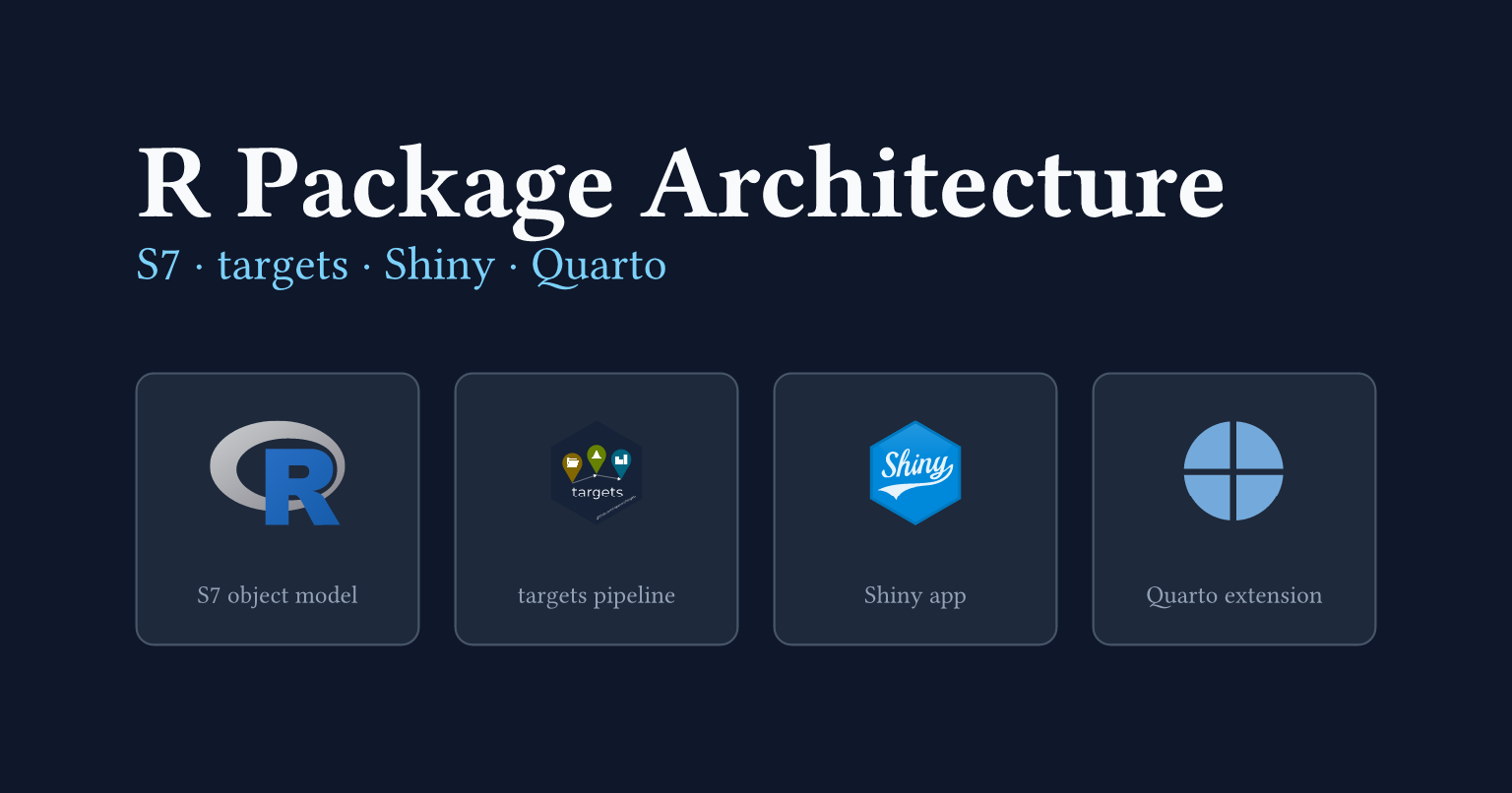
The package rests on four parts that compose cleanly.


Each pillar is a distinct tool with a different job. S7 defines the typed data structures the rest of the package operates on. targets is a build system: it caches intermediate results and only re-runs steps whose inputs have changed. Shiny turns R functions into an interactive web app, with no JavaScript needed. Quarto renders documents from a single source file: HTML pages, PDFs, slide decks, all from the same prose and code.
The S7 objects are the currency that flows between the four parts. The pipeline, the report, and the Shiny app all pass them around and call the same generics.
3 An S7 object model
R is a functional language, but it lets you define your own types. A class is a named structure with rules: it says what fields a value must have, what types those fields must be, and what makes a value valid. Once you have a class, you can write functions whose behaviour changes depending on what type of object you pass them. That is the whole idea.
S7 is the R Consortium’s current answer to “how should R do this”. It replaces the older S3 and S4 systems with a cleaner API: you declare properties (the fields), a validator (the rules), and a constructor (how to build one). You call @ to read a field, just like $ for a list.
The package has three classes. Dataset wraps a data.frame and records when it was created. AnalysisResult holds the summary table and method name produced by one analysis run. Project owns a dataset and an ordered list of results.
R/aab-classes.R
Dataset <- S7::new_class(
  name = "Dataset",
1  properties = list(
2    data = S7::class_any,
3    name = S7::new_property(class = S7::class_character, default = ""),
    created = S7::new_property(class = S7::class_any, default = NULL)
  ),
4  validator = function(self) {
    if (!is.null(self@data) && !is.data.frame(self@data)) {
      return("@data must be a data.frame or NULL")
    }
    if (length(self@name) != 1L) {
      return("@name must be a single string")
    }
    NULL
  },
5  constructor = function(data = NULL, name = "") {
    S7::new_object(
      S7::S7_object(),
      data = data,
      name = name,
      created = Sys.time()
    )
  }
)- 1
- Properties are typed slots; every instance must carry a value for each.
- 2
-
class_anyaccepts any R object with no type check. - 3
-
new_property()adds a class constraint and a default value; omittingnamegives"". - 4
-
All invariants go in
validator; returning a string fails construction with that message. - 5
-
The constructor stamps
createdautomatically; callers only supplydataandname.
Verbs are S7 generics. A generic is a function that looks at the type of its first argument and calls the right implementation. You define the generic once, then attach a separate implementation for each class. Generics go in aaa-generics.R, before the class files, so the implementations can attach to them when R loads the package.
R/aaa-generics.R
- 1
-
The dispatch argument: S7 picks the method based on the class of
object. - 2
-
Must call
S7_dispatch()in the body; this triggers method lookup and execution.
The Project method delegates to the Dataset method, stores the result, and updates the timestamp.
R/analyse.R
- 1
-
Attaches a method to the
analysegeneric specifically forProjectobjects. - 2
-
Delegates to the
Datasetmethod by passingobject@data; no logic is duplicated. - 3
-
S7 slot assignment uses
@<-, the same accessor as reading (@).
One more thing worth keeping: the filter() generic uses a search-path fallback so the package’s own filter() method works on Dataset objects while dplyr’s filter() still works on data frames. The default method walks the search path and delegates to the next plain function of the same name.
One generic, many callers: analyse(dataset) and analyse(project) look identical at the call site. S7 routes each to the right implementation. No type-checking if branches anywhere in the calling code.
4 A config-driven pipeline
Most people who run an analysis are not R developers. They know what data they have and what question they want to answer, but they should not need to open a .R file to say so.
A YAML config makes this possible. It reads like plain English: here is the data file, here are the analyses to run, here is what the report should be called. No R syntax, no package knowledge, no risk of accidentally breaking the pipeline logic. The package owns the code; the config owns the decisions.
R developers who want more control are not forced through the config. They can call Dataset(), analyse(), and the rest of the verbs directly, compose them however they like, and build their own pipeline. The config-driven workflow is a convenience layer on top, not a gate.
generate_pipeline() validates the config, fills a whisker/Mustache template, and writes a _targets.R file. run_pipeline() calls targets’ tar_make() to execute it. report_pipeline() renders the Quarto report from the store.
pipeline-config.yml
data:
  file: demo.csv
  name: demo
analyses:
  summary:
    method: describe
  pairs:
    method: correlate
report:
  title: "Acme Analysis Report"
  formats:
    - acme-html
The template is the interesting part. Each analysis in the config becomes one targets target. The whisker {#analyses} ... {{/analyses}} section expands once per entry.
inst/templates/_targets.R
list(
  tar_target(input_file, "{{{data_file}}}", format = "file"),
  tar_target(
    dataset,
    acme.toolkit::Dataset(data = utils::read.csv(input_file), name = "{{{data_name}}}")
  ){{#analyses}},
  tar_target(
    {{name}},
    acme.toolkit::analyse(dataset, method = "{{method}}")
  ){{/analyses}}
)
The leading comma belongs at the start of each repeated block, after the always-present dataset target. This avoids a trailing comma in the generated list, which would be a parse error.
The config hash is written into the file header at generation time. If the config drifts from what was used to generate the pipeline, a later run can warn about it.
5 A bundled Quarto extension
Branding lives in exactly one place: a Quarto extension under inst/_extensions/acme/. One _extension.yml defines three formats.
inst/_extensions/acme/_extension.yml
title: Acme
version: 0.1.0
quarto-required: ">=1.5.0"
contributes:
  metadata:
    project:
      brand: _brand.yml
  formats:
    common:
      filters:
        - filters/prose-divs.lua
        - filters/copyright-year.lua
      toc: true
      number-sections: true
    html:
      theme: [cosmo, brand, acme.scss]
      embed-resources: true
      title-block-banner: true
    typst:
      papersize: a4
      margin: {top: 2.5cm, bottom: 2.5cm, left: 2cm, right: 2cm}
    revealjs:
      theme: [default, brand, revealjs/theme.scss]
      embed-resources: true
A document opts in with one line.
format: acme-htmlColours, fonts, and logos live in _brand.yml. Quarto’s native brand support feeds them into every format, so the SCSS files only add layout rules.
The extension ships inside the package at inst/_extensions/acme/. When the pipeline is generated, .install_acme_extension() copies it into the project directory. Quarto resolves _extensions/ from the document’s directory, so the copy must be local. Re-skinning the whole system means editing three files: _brand.yml, acme.scss, and revealjs/theme.scss.
One extension, three formats: acme-html, acme-typst, and acme-revealjs all draw from the same _brand.yml. Swap the palette once and every output follows.
6 A modular Shiny app
The Shiny app reuses the package’s analysis code. It does not re-implement it. The modules call analyse(), the same generic the batch pipeline calls.
Shiny modules exist to solve a scoping problem. In a plain Shiny app, every input and output shares a single namespace, so names clash as the app grows. A module wraps a piece of UI and its server logic into an isolated unit with its own namespace. You can drop it into any app by calling two functions: one for the UI, one for the server.
That last point matters here. The three modules are not just internal implementation details of this package’s bundled app. They are the public interface for other Shiny apps. If you already have a Shiny app and you want to add an acme.toolkit analysis panel to it, you call mod_analysis_ui() and mod_analysis_server() and you are done. No copy-pasting, no re-implementing the analysis logic.
Modules as a public API: the three modules ship as the embeddable interface for any Shiny app. Drop them into an existing app the same way you drop them into the bundled one.
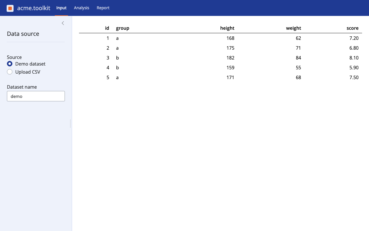
mod_input loads a CSV and writes a Dataset into shared state. mod_analysis reads the dataset, runs analyse(), and writes the result. mod_report reads the result and offers a Quarto report as a download.
The top-level server owns the shared state and passes it into each module.
R/app_server.R
app_server <- function(input, output, session) {
1  dataset <- shiny::reactiveVal(NULL)
  result <- shiny::reactiveVal(NULL)

  mod_input_server("input", dataset = dataset)
  mod_analysis_server("analysis", dataset = dataset, result = result)
  mod_report_server("report", result = result)

  invisible(NULL)
}- 1
- Shared state lives here. Modules never reach into each other.
The data flows in a straight line.


Inside mod_analysis, the call is simply:
R/mod_analysis.R
shiny::observeEvent(input[["run"]], {
  ds <- dataset()
  if (is.null(ds)) {
    shiny::showNotification("Load a dataset first.", type = "warning")
    return()
  }
1  result(analyse(ds, method = input[["method"]]))
})- 1
-
Same
analyse()generic as the pipeline. No logic is duplicated.
The module does not know how analyse() works. If you update the analysis logic inside the package, both the pipeline and the Shiny app pick it up.
7 Putting it all together
Depending on who you are, you interact with the package differently.
If you are a clinician or analyst who does not write R, you fill in a YAML config file. You say which data to use, which analyses to run, and what to call the report. Then you call run_pipeline(). A branded HTML or PDF report appears in your project folder. You never open a .R file.
If you want to explore the data interactively, you open the Shiny app with run_app(). You upload a CSV, pick an analysis method, and download the result. The app calls the same analyse() function the batch pipeline calls.
If you are an R developer who wants to extend or customise the analysis, you work directly with the S7 classes and generics. You write a new method, add a property, or compose the verbs in a custom script. The change flows into the pipeline, the Shiny app, and the report without touching any of those.
That is what the architecture is for. The same analysis logic runs in a terminal, in a browser, and in a PDF. Keeping it in one place is the only way to keep it consistent.
The full working package is at mcanouil/demo-r-package-shiny-quarto. It builds clean with zero errors, warnings, and notes.
Happy coding!
Reuse
Citation
@misc{canouil2026,
  author = {CANOUIL, Mickaël},
  title = {R {Package} {Architecture:} {Shiny,} {Quarto,} Targets, and
    {S7}},
  date = {2026-07-01},
  url = {https://mickael.canouil.fr/posts/2026-07-01-r-package-shiny-quarto/},
  langid = {en-GB}
}