Gribouille 0.5.0: Native Density, and Scales Keyed by Aesthetic
Gribouille 0.5.0 brings native kernel density estimation to Typst: densities, violins, two-dimensional densities, ridgelines, and a LOESS smoother, all computed in pure markup. It also rewrites the scale system so the per-aesthetic scale-* constructors collapse into a single keyed scales(), the largest breaking change of the release. Streamgraphs, bump charts, and waffle charts join the roster too.
Another Gribouille release. Gribouille 0.5.0 is all about density but not just that. Kernel density estimation runs natively now, in pure Typst, so densities, violins, two-dimensional densities, and ridgeline plots all draw without leaving the document. The LOESS smoother lands in the same pass. In addition to density, the one thing to watch when you upgrade is the scale system: the per-aesthetic scale-* constructors collapse into a single keyed scales(), so scale-colour-viridis-d() becomes scales(colour: scale-viridis-d()).
NoteAt a glance
Gribouille 0.5.0 on Typst Universe: #import "@preview/gribouille:0.5.0": *.
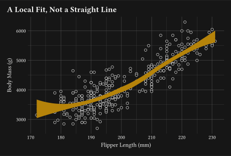
geom-smooth() gains method: "loess" with span and degree control, next to the existing "lm".
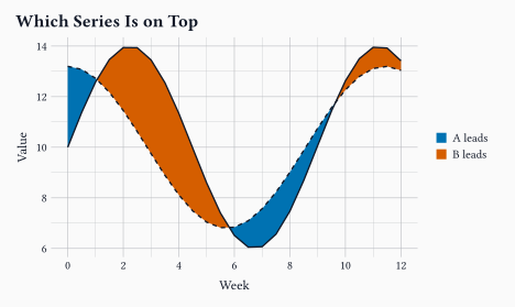
geom-beeswarm() lays overplotted points into a deterministic swarm, and stat-difference shades the band between two series by which one is on top.
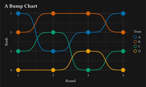
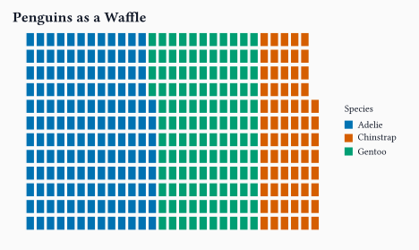
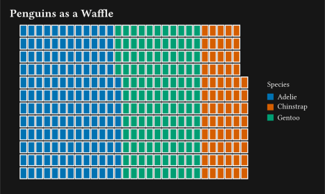
Streamgraphs (position-stack(offset:)), bump charts (stat-connect(connection: "sigmoid")), and waffle charts (stat-waffle) join the chart types.
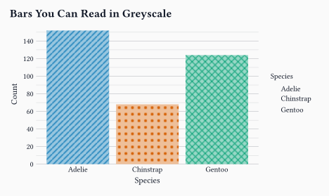
Fills accept native Typst tiling patterns, both as a fixed fill: and through scale-manual(values:).
Breaking: the per-aesthetic scale-* constructors collapse into a keyed scales(); the aesthetic comes from the key, so scale-colour-viridis-d() becomes scales(colour: scale-viridis-d()) and scale-x-log10() becomes scales(x: scale-log10()). plot(scales:) now takes only the scales() dictionary.
Breaking:linetype defaults to auto on the line-drawing geoms, honouring a mapped linetype scale instead of pinning "solid".
Every figure in this post is a real, freshly compiled plot.
1 Breaking changes
Two changes need your attention before your old code compiles. Neither changes what a plot looks like, only how you spell the scales.
WarningMigrate these names
The per-aesthetic scale-* constructors are gone. Wrap the aesthetic-agnostic constructor in scales() and let the key carry the aesthetic: scale-colour-viridis-d() becomes scales(colour: scale-viridis-d()), and scale-x-log10() becomes scales(x: scale-log10()). plot(scales:) takes only the scales() dictionary, no positional array, and expand-limits() returns an aesthetic-keyed dictionary.
linetype now defaults to auto on geom-segment, geom-curve, geom-spoke, geom-errorbar, geom-errorbarh, geom-linerange, and geom-pointrange. A mapped linetype scale is honoured instead of being overridden by a pinned "solid". Pass linetype: "solid" on the geom if you want the old fixed look.
There is one more change, but it is internal. Every constructor dictionary now stores its concrete type under a single name: key. This only matters if you pattern-match the dictionaries a constructor returns; the way you call them in a plot is unchanged.
2 A keyed scales()
The old scale names spelled the aesthetic into the function: scale-colour-viridis-d, scale-x-log10, scale-fill-manual. That meant one constructor per aesthetic, and a long list of near-duplicates. Now there is one aesthetic-agnostic set, and the aesthetic comes from the key you bind it to inside scales(), exactly like guides().
scales() is keyed by aesthetic and named only. A stray positional argument is rejected.
2
scale-x-log10() is now scale-log10() under the y key. The same constructor serves the x axis.
3
scale-colour-okabe-ito() is now scale-okabe-ito() under the colour key. Use it under fill for a fill scale.
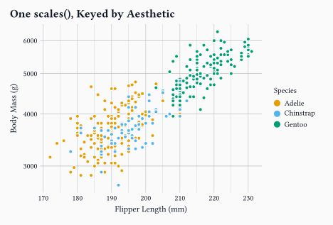
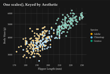
scales() is more than a tidy wrapper. You could hand plot() a plain named dictionary, (colour: scale-okabe-ito()), and it would look the same. The difference is that scales() checks every entry as it binds it, before the plot draws. A positional argument, an aesthetic key that does not exist, or a value that is not a scale spec each stops with a clear message that lists the valid names. A plain dictionary would keep a misspelled key like colur: and quietly drop the scale, so the plot would render with the wrong colours and no error to point at. An unknown argument to a scale-* constructor is caught at the same moment, reported with the keys that scale accepts for that aesthetic.
A dictionary swallows a typo; scales() rejects it: a wrong aesthetic key or a non-scale value fails loudly instead of drawing a misleading plot.
3 Native density
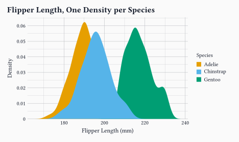
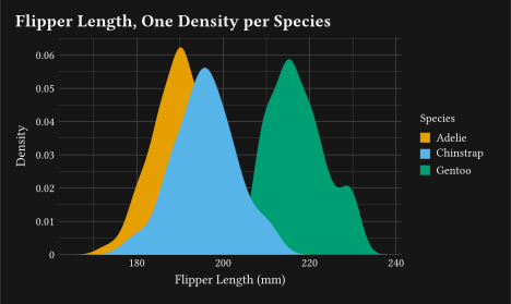
Density estimation is the heart of this release. geom-density() evaluates a Gaussian kernel on a grid and draws the smooth curve, all in Typst, with no external runtime. The bandwidth is chosen by Silverman’s rule and tuned with adjust; trim cuts the curve to the data range.
#plot( data: penguins, mapping: aes(x:"flipper-len", fill:"species"), layers:(1 geom-density(alpha:0.5, adjust:1),), scales: scales(fill: scale-okabe-ito()), labels: labels( title:"Flipper Length, One Density per Species", x:"Flipper Length (mm)", y:"Density", fill:"Species",), theme: theme-minimal(), width:12cm, height:7cm,)
1
adjust scales the automatic bandwidth; bw pins it outright, and trim: true clips the curve to the observed range. Map aes(weight: ...) for a weighted density.
The stat exposes the usual after-stat columns, _density, _count, _scaled, and _n, so you can map y to a count instead of a density when that reads better.
4 Violins and beeswarms
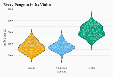
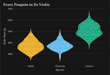
A violin is the same density, mirrored and turned on its side. geom-violin() draws one silhouette per group, normalised by scale. geom-beeswarm() spreads the raw points into a deterministic, density-shaped swarm, a reproducible alternative to jitter. Layer the swarm over the violin and every penguin sits inside its own silhouette.
scale: "width" gives every violin the same maximum width; "area" (the default) equalises area, and "count" scales width by the group size. Overlapping groups dodge with position: "dodge".
2
The swarm spreads the points on the discrete axis directly, no as-factor needed; position-beeswarm(width:, adjust:) tunes the spread.
5 Two dimensions at once
For a scatter that is too dense to read, a two-dimensional density shows where the mass sits. geom-density-2d-filled() shades filled iso-bands of the joint density; geom-density-2d() draws the iso-lines instead.
bw sets the per-axis bandwidth (a number or an (x, y) pair) and n the grid resolution. Map fill: after-stat("_level") on geom-density-2d() to shade the lines by level.
6 Ridgelines
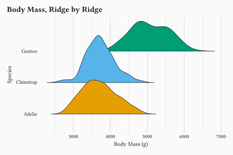
When a plain overlap gets crowded, a ridgeline offsets each density up the panel. geom-density-ridges() draws one ridge per y level, with heights normalised across levels so they compare fairly.
scale is measured in y-level units: 1 lets a ridge just reach the next baseline, and a larger value lets them overlap. The stat supplies the height channel the geom draws from, so keep the default stat.
2
The discrete y-scale needs a little headroom on top so the tallest ridge is not clipped.
7 A LOESS smoother
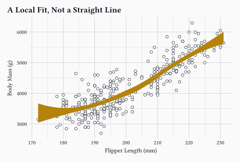
Until now, fitted straight lines were the only smoothers geom-smooth() could draw (method: "lm"). Now geom-smooth() also takes method: "loess", a local polynomial fit with a pointwise confidence band.
#plot( data: penguins, mapping: aes(x:"flipper-len", y:"body-mass"), layers:( geom-point(size:2pt, alpha:0.5),1 geom-smooth(method:"loess", span:0.75, degree:2),), labels: labels( title:"A Local Fit, Not a Straight Line", x:"Flipper Length (mm)", y:"Body Mass (g)",), theme: theme-minimal(), width:12cm, height:8cm,)
1
span sets the fraction of points in each local window, and degree the local polynomial order (0, 1, or 2). The default method: "lm" still draws the straight-line fit.
8 Difference bands
stat-difference shades the band between two series by which one is on top. Feed it ymin and ymax, map fill: after-stat("_sign"), and it splits the ribbon at every crossover, filling the gap in the colour of whichever line leads.
The two series enter as ymin and ymax; fill: after-stat("_sign") colours each run by which one is higher.
2
levels: names the two states, and exact crossovers are inserted as shared vertices so the bands meet cleanly.
9 Pattern fills
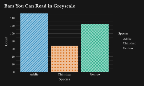
A fill no longer has to be a flat colour. When colour/fill is not enough or is too much, a pattern can carry the information instead which helps improve accessibility and printability. Fills now accept native Typst tiling patterns, both as a fixed fill: and through scale-manual(values:), and the legend swatches draw the patterns too. This is what keeps a bar chart readable once it is printed in black and white.
Each pattern is a plain Typst tiling: a full-tile background box, then the marks on top. A tiling works anywhere a colour does.
2
scale-manual binds one pattern per level. The legend swatches render the patterns, not flat colours.
10 New chart types
A few new stats and positions turn familiar geoms into charts they could not draw before.
10.1 Streamgraphs
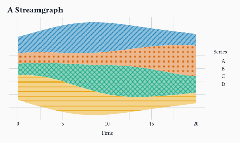
position-stack gains a streamgraph baseline. Pass offset: "silhouette" to centre each stack on zero, or offset: "wiggle" for the Byron-Wattenberg baseline, and a stacked geom-area() becomes a streamgraph.
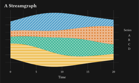
Each band gets its own tiling pattern, so the streamgraph stays legible without relying on colour alone.
2
offset: "wiggle" gives the classic streamgraph baseline instead; "none" (the default) stacks from zero as before.
10.1.1 Bump charts
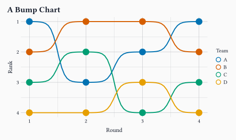
stat-connect gains a "sigmoid" connector. Paired with geom-line() and a reversed y-scale, it draws a bump chart, one smooth S-curve between each pair of ranks.
rows sets the grid height in cells and columns grow to hold the total; the page-coloured stroke keeps the cells apart. Map weight instead when the data is already counted, one row per group.
11 Agents and plugins
Gribouille ships an installable agent skill that teaches a coding assistant to write correct plots, checking every argument against the documentation. It installs with:
npx skills add mcanouil/gribouille
The repository doubles as a Claude Code plugin marketplace, so you can wire the same skill into Claude Code:
As always, a good share of the release is fixes rather than features.
Errors fail loudly now: an unknown aesthetic, theme key, stat, or column stops with a clear message instead of a misleading plot.
The biggest is stricter validation. An unknown aes() aesthetic, such as the US spelling color, now fails with the list of valid aesthetics instead of drawing an empty plot. theme() rejects a misspelled element key, an unknown stat or scale transform fails with a clear message rather than rendering as identity, and mapping an aesthetic to a missing column names the column and lists the ones that exist.
Two rendering fixes are worth calling out. Abutting opaque fills, such as tiles, hexes, and stacked bars, are now stroked with their own fill colour, which removes the hairline seams that antialiasing used to bleed through between them. And stat-quantile drops its cubic pair enumeration for an exact O(n^2 log n) search, so geom-quantile scales to thousands of rows.
Facets and compositions also gain spacing control. facet-wrap and facet-grid take a gutter argument, and a new theme(panel-spacing:) default sets the gap for both axes at once (a length, or a (x:, y:) dictionary); compose’s gutter now accepts the same dictionary form.
13 Wrap-up
Kernel density estimation, in pure Typst, plus one keyed scales() in place of a constructor per aesthetic.
Next on the list is more geoms and more worked examples. If you run into something unexpected, the issue tracker is the right place for it.
Gribouille is an unfunded spare-time project, and the API is still settling. Bug reports and ideas are very welcome on the issue tracker. Pull requests are not being accepted for now, for the reasons set out in the launch post. Thanks in advance for your patience.